A beginner’s tutorial for your first Machine Learning project using Charmed Kubeflow
shrishtikarkera
on 17 December 2024
Wouldn’t it be wonderful to wake up one day with a desire to explore AI and machine learning, only to find a well-crafted, simple, and beginner-friendly tutorial that covers all of the crucial core elements you need to build your very first model? Well, you’ve come to the right place!
The goal of this guide is to show you how to develop a model capable of classifying different species of Iris flowers based on their characteristics, such as sepal length and petal width. This will help you to learn the fundamentals of building and deploying machine learning models, which will serve you well in more complex projects down the line. In this guide, we will walk through how to build a model to solve the Iris Classifier problem, a famous classification example in the machine learning community.
Overview
The Iris Classifier problem challenges us to build a model that can accurately categorize Iris flowers into three species: “setosa”, “versicolor”, and “virginica”. By the end of this tutorial, you’ll have a working machine learning model trained on the Iris dataset, ready to make predictions.
This comprehensive tutorial covers the following topics:
- Writing Basic ML Code: Learn how to write fundamental machine learning code using popular Python libraries.
- Converting Notebooks to YAML: Understand the steps to convert a Jupyter notebook into a YAML file.
- Creating a Pipeline: Discover how to build a pipeline from the YAML file and initiate a run.
- Model Inferencing: Gain insights into performing inference with the machine learning model stored in our MinIO bucket.
Whether you’re a newcomer to the field or looking to solidify your understanding of core ML principles, this tutorial will provide you with the hands-on experience you need to start your machine learning journey.
This tutorial uses Charmed Kubeflow as a project platform, as it is a straightforward, easy-to-use choice for beginners venturing into AI and machine learning. Charmed Kubeflow is built on Kubernetes (microK8s) and has a user-friendly deployment process and integrated suite of tools that streamline the various stages of machine learning projects, making it an ideal starting point for beginners.
Since it automates many operational tasks, it enables beginners to focus on learning rather than infrastructure management. This also makes it highly scalable, by accommodating growing needs without the complexities of managing infrastructure.
1. Environmental Setup
This tutorial requires you to install Charmed Kubeflow and its required components. The process is quick and easy, however going over them is outside of the scope of this tutorial. Lucky for you and other newcomers, there’s a comprehensive and easy-to-follow guide available on the Charmed Kubeflow documentation page.
The minimum requirements to run Charmed Kubeflow are:
- Ubuntu 20.04 (Focal) or later.
- A host machine with at least a 4-core CPU processor, 32GB RAM and 50GB of disk space available.
I launched an AWS t3.xlarge instance configuration with 8 vCPUs and 150 GB of volume, but you are free to choose other options that fit your needs. Generally this is more than enough to get started with your first project. After installing kubeflow and configuring the dex-auth login credentials, configure minIO for storing our model, artifacts, datasets, etc. Installing these should be quick and efficient, taking less than an hour. The discourse pages linked at the bottom of these guides contain helpful resources and tips for dealing with any potential issues you may face.
1.1 Introduction to the Kubeflow environment:
After setting up the environment successfully, we can now access the dashboard at https://10.64.140.43.nip.io/ or at the IP that was output by “Access the dashboard” step.
Diagram 1.1 a: Kubeflow central dashboard
This step involves launching a JupyterLab notebook to begin writing Python code. Jupyter Notebook is an interactive Python-based computing platform that enables data scientists to combine code, visualizations, video, images, text and other media into highly interactive data science projects.
In our JupyterLab notebook we will use the standard SciPy image and enable access to Kubeflow pipelines through the advanced options. You can see in the below image how I launched a Jupyter notebook using the base image: scipy (standard).
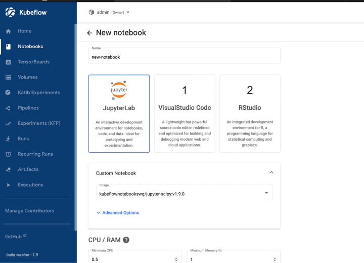
Diagram 1.1 b: Kubeflow notebooks tab
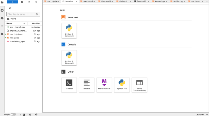
Diagram 1.1 c: Launched notebook options
We can also login to the MinIO dashboard with the credentials obtained from “Access the dashboard IP address” step.
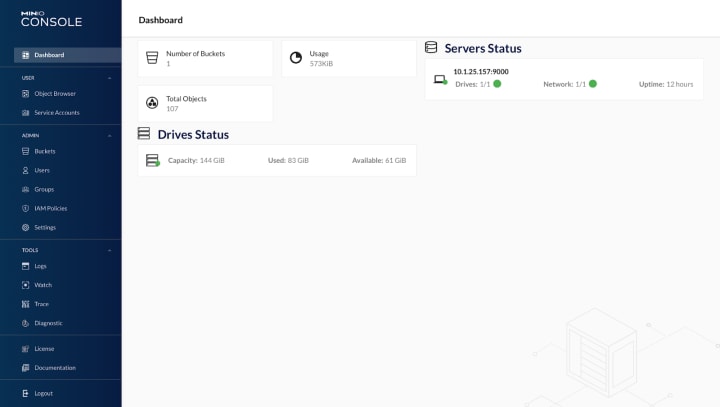
Diagram 1.1 d: MinIO dashboard
2. Machine learning code
In this section, we will analyse the problem statement and start writing the machine learning code. We will explore a fundamental example often referred to as the “hello world” of machine learning: the Iris classification problem.
2.1 The Iris classification problem
The Iris classification problem is perhaps the most famous project example problem in beginner machine learning. This problem involves classifying iris flowers into one of three species (Setosa, Versicolor, and Virginica) based on four measurable characteristics, which are the flower’s sepal length, sepal width, petal length and petal width (all measured in centimeters).
This dataset consists of 50 samples from each of the three species, resulting in a total of 150 samples.
The iris problem is perfect as a beginner project, as it’s an easy-to-understand, real-world example with clear use cases beyond its data set, and it teaches beginners to work with multivariate data and continuous features to make clear categorizations or classifications. The data set is also freely available for download, and deals with some of the most fundamental concepts in machine learning and problem solving.
Your project will begin by importing this dataset from the sklearn datasets.
Let’s begin by understanding what the iris dataset looks like. Iris is a class of flower. In the standard iris dataset, sklearn.datasets.load_iris(), there are 3 target classes: Iris Setosa, Iris virginica, and Iris versicolor. The job of the classifier is to predict the class of the flower given the input. The input has 4 parameters – sepal length (cm),sepal width (cm), petal length (cm), petal width (cm).
The most important things that we’ll be looking at here are the input and output data structures, because these indicate what category of algorithms the problem falls under, like linear regression, computer vision, language translation, and so on.
So for our purposes, we need a model capable of predicting the class to which a flower belongs, which can be framed as a logistic regression problem.
Let’s delve into the reasoning behind this approach.
2.1.1 What is logistic regression and why do we use it?
In order to begin classifying the iris flowers, we need to first have a basic understanding of linear and logistic regression. The iris example is a little challenging, as it involves a four-dimensional input and three outputs, and so in the interest of simplicity and beginner friendliness let us consider a simpler, more relatable scenario: the relationship between weight and obesity. Instead of flowers, we can use mice: we can define 𝑥 as the weight of a mouse and 𝑦 as a binary indicator of whether the mouse is obese.
We can think of logistic regression as a concept similar to linear regression which we are all familiar with, but with one key difference: logistic regression predicts binary outcomes (‘true’ or ‘false’) rather than continuous values like linear regression does.

Diagram 2.1.1 a: Logistic regression mice example
In linear regression, we fit a line through the data but in logistic regression, we fit an S-shaped curve which tells you whether the mouse is obese based on its weight.
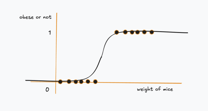
Diagram 2.1.1 b: Logistic regression curve
If we add a new mouse to our data set and it is heavy, there’s a strong likelihood that it is obese. If it has an average weight, there’s a 50% chance of obesity, while a light mouse has a very low probability of being obese.
Although logistic regression gives us the probability of whether the mouse is obese or not, it’s mostly used for classification. For example, if the output probability is greater than 50%, we classify it as obese, else not obese. We can also develop more complex models where factors like weight, genotype, age, and others influence whether a mouse is obese or not.
Another difference between linear and logistic regression is how the line fits on the data points. In linear regression, we consider the line with minimum sum of squares of the residuals and in logistic regression, we use something known as “maximum likelihood”. This is done by calculating the likelihood of all the mice and then picking the curve with maximum likelihood.

Diagram 2.1.1 c: Comparison between linear and logistic regression
The logistic regression equation looks like this –
Even though it may seem like there’s no actual training happening to consider logistic regression as a machine learning technique, it still learns from the data to fit the curve as shown in diagram 2.1.1 c.
For the purpose of our code, we will use the LogisticRegression classifier from the sklearn library to fit the model on the training data and use the joblib library to dump the final model weights into the MinIO bucket or the local folder.
2.1.2 The code
A typical machine learning workflow consists of the following steps:
- Load the data
- Pre-process the dataset
- Train the model
- Evaluate the model
- Perform inference on new data
In this particular instance, we do not require extensive pre-processing because we extracted the dataset from the sklearn library and it is already clean. Therefore, after loading the iris dataset, our pre-processing step will involve splitting the data into training and testing sets. Typically, we divide the dataset into a training set and a test set, as indicated by their names: the training set is used for training the model, while the test set is reserved for evaluating it. During the evaluation process, we input the test data without revealing the corresponding outputs, and we calculate the error between the actual outputs of the test set and those produced by the model using the logistic regression equation.
Let’s begin by importing the datasets and libraries that we need for our project:
import pandas as pd
import os
from sklearn import datasets
from minIO import minIO

 # Load dataset
def prepare_data():
    iris = datasets.load_iris()
    df = pd.DataFrame(iris.data, columns=iris.feature_names)
    df['species'] = iris.target
    return df

# Split the data into training and testing data
def train_test_split(df):
    target_column = 'species'
    X = df.loc[:, df.columns != target_column]
    y = df.loc[:, df.columns == target_column]

    X_train, X_test, y_train, y_test = train_test_split(X, y, test_size = 0.3,stratify = y, random_state=47)
    return X_train, X_test, y_train, y_test

# Train the model
def train_model(X_train, y_train):
    iris_model = LogisticRegression(max_iter=200)
    iris_model.fit(X_train,y_train)
    joblib.dump(iris_model, 'iris_model.pkl')

df = prepare_data()
X_train, X_test, y_train, y_test = train_test_split(df)
train_model(X_train, y_train)
3. Building KubeFlow pipelines from JupyterLab notebooks
We will now convert our JupyterLab notebook code into a YAML file to create a Kubeflow pipeline as it brings several important benefits for machine learning workflows. Kubeflow pipelines enhance reproducibility by ensuring consistent execution of experiments, while also allowing for easy scalability to manage larger datasets and complex computations. Automation of tasks reduces manual intervention and the risk of errors, and better versioning helps track changes and optimize models over time.
Additionally, Kubeflow pipelines integrate seamlessly with various tools and services, facilitating streamlined workflows for data preprocessing, model training, and deployment.
We will use kfp to convert our jupyterlab code to a pipeline.
3.1 Using Kubeflow pipelines
By allowing us to create reusable and scalable pipelines, kfp enhances the reproducibility and efficiency of our machine learning projects. In this section, we’ll dive into how to convert our existing machine learning code into a Kubeflow pipeline, making it easier to manage and execute our workflows effectively.
Now, we will convert our functions to components and link these components together into a pipeline and compile it all into a YAML file. This generated YAML file is then used to create a new pipeline run using the GUI.
We can also pass our model artifacts like return values and variables through the different functions, but this advanced technique is out of scope for this beginner tutorial. However, it’s worth learning later on to use in more complex projects.
3.1.1 Final code
We’re using MinIO for storing our dataset and model. It is an object storage platform like S3 storage in AWS but MinIO has direct integration with Kubeflow when we use Charmed Kubeflow. Next, we’ll start loading data from the library and upload it in a MinIO bucket named “mlpipeline”.
@component(
    Packages_to_instal = ["pandas", "numpy", "scikit-learn", "minIO"],
    base_image="python:3.9",
)
def prepare_data():
    import pandas as pd
    import os
    from sklearn import datasets
    from minIO import minIO
    # Load dataset
    iris = datasets.load_iris()
    df = pd.DataFrame(iris.data, columns=iris.feature_names)
    df['species'] = iris.target

    df = df.dropna()


    minIO_client = minIO(
        "10.152.183.213:9000",
        access_key = "minIO",
        secret_key = "minIO123",
        secure = False
    )
    minIO_bucket = "mlpipeline"
    df.to_csv('final_df.csv', index=False)
    minIO_client.fput_object(minIO_bucket,"final_df.csv","final_df.csv")
Now, let’a split the data into X – train/test and y – train/test
@component(
    packages_to_install=["pandas", "numpy", "scikit-learn", "minIO"],
    base_image="python:3.9",
)
def train_test_split():
    import pandas as pd
    import numpy as np
    import os
    from sklearn.model_selection import train_test_split
    from minIO import minIO
    minIO_client = minIO(
        "10.152.183.213:9000",
        access_key="minIO",
        secret_key="minIO123",
        secure=False
    )
    minIO_bucket = "mlpipeline"

    minIO_client.fget_object(minIO_bucket,"final_df.csv","final_df.csv")
    final_data = pd.read_csv('final_df.csv')

    target_column = 'species'
    X = final_data.loc[:, final_data.columns != target_column]
    y = final_data.loc[:, final_data.columns == target_column]

    X_train, X_test, y_train, y_test = train_test_split(X, y, test_size=0.3,stratify = y, random_state=47)

    np.save('X_train.npy', X_train)
    minIO_client.fput_object(minIO_bucket,"X_train.npy","X_train.npy")
    np.save('X_test.npy', X_test)
    minIO_client.fput_object(minIO_bucket,"X_test.npy","X_test.npy")
    np.save('y_train.npy', y_train)
    minIO_client.fput_object(minIO_bucket,"y_train.npy","y_train.npy")
    np.save('y_test.npy', y_test)
    minIO_client.fput_object(minIO_bucket,"y_test.npy","y_test.npy")
Now, lets build a component for training the Logistic Regression model using sklearn
@component(
    packages_to_install=["pandas", "numpy", "scikit-learn", "minIO", "joblib"],
    base_image="python:3.9",
)
def training_basic_classifier():
    import pandas as pd
    import numpy as np
    import os
    from sklearn.linear_model import LogisticRegression
    from minIO import minIO
    import joblib
    minIO_client = minIO(
        "10.152.183.213:9000",
        access_key="minIO",
        secret_key="minIO123",
        secure=False
    )
    minIO_bucket = "mlpipeline"

    minIO_client.fget_object(minIO_bucket,"X_train.npy","X_train.npy")
    X_train = np.load('X_train.npy',allow_pickle=True)
    minIO_client.fget_object(minIO_bucket,"y_train.npy","y_train.npy")
    y_train = np.load('y_train.npy',allow_pickle=True)

    iris_model = LogisticRegression(max_iter=200)
    iris_model.fit(X_train,y_train)
    joblib.dump(iris_model, 'iris_model.pkl')
    minIO_client.fput_object(minIO_bucket,"models/iris_model.pkl","iris_model.pkl")
The component outlined below will retrieve the model from MinIO and execute an inference service using the KServe InferenceService client, a widely recognized inference component within Kubernetes.
@component(
    packages_to_install=["kserve"],
    base_image="python:3.9",
)
def model_serving():
    from kubernetes import client
    from kserve import KServeClient
    from kserve import constants
    from kserve import utils
    from kserve import V1beta1InferenceService
    from kserve import V1beta1InferenceServiceSpec
    from kserve import V1beta1PredictorSpec
    from kserve import V1beta1SKLearnSpec
    import os

    namespace = utils.get_default_target_namespace()

    name='iris-model'
    kserve_version='v1beta1'
    api_version = constants.KSERVE_GROUP + '/' + kserve_version

    isvc = V1beta1InferenceService(api_version=api_version,
                                   kind=constants.KSERVE_KIND,
                                   metadata=client.V1ObjectMeta(
                                       name=name, namespace=namespace, annotations={'sidecar.istio.io/inject':'false'}),
                                   spec=V1beta1InferenceServiceSpec(
                                   predictor=V1beta1PredictorSpec(
                                   service_account_name="sa-minIO-kserve",
                                   sklearn=(V1beta1SKLearnSpec(storage_uri="s3://mlpipeline/models/iris_model.pkl")))))
Now, to the final act of assembling all of our components into a pipeline:
@pipeline(
    name="iris-pipeline"
)
def iris_pipeline():
    prepare_data_task = prepare_data()
# Split data into Train and Test set
    train_test_split_task = train_test_split()
    train_test_split_task.after(prepare_data_task)

    # Model training
    training_basic_classifier_task = training_basic_classifier()
    training_basic_classifier_task.after(train_test_split_task)

    model_serving_task = model_serving()
    model_serving_task.after(training_basic_classifier)


# Compile the pipeline
if __name__ == '__main__':
    compiler.Compiler().compile(
        pipeline_func=iris_pipeline,
        package_path=iris_pipeline.yaml'
    )
This process generates an iris_pipeline.yaml file in our local directory, which we can use to create a Kubeflow pipeline. YAML files are widely utilized for configuration purposes and in applications where data is stored or transmitted. So, we’ll use this file to create a pipeline.
Next, we will navigate to the Pipelines tab in our Kubeflow dashboard to upload the file. To initiate a run, we must first create an experiment from the Experiments tab.
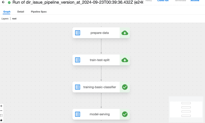
Diagram 3.1.2 a: Iris classification pipeline
After running the pipeline, we can see the model.pkl (weights file) in MinIO under the models folder in the mlpipeline bucket:
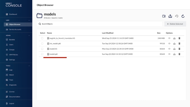
Diagram 3.1.2 b: Iris classification model in MinIO bucket
4. Inference with Kserve InferenceService
Now that we have created the inference service, you should see the model in the inferenceservices list:
kubectl get inferenceservices iris-model -n admin
You should see the following output
Next, we will create an input json file to request an inference:
cat <<EOF > "./iris-input.json"
{
  "instances": [
    [6.8,  2.8,  4.8,  1.4],
    [6.0,  3.4,  4.5,  1.6]
  ]
}
EOF
Now, we can directly curl the InferenceService with the URL obtained from the status:
curl -v -H "Content-Type: application/json" http://sklearn-iris.kserve-test.${CUSTOM_DOMAIN}/v1/models/sklearn-iris:predict -d @./iris-input.jsonYou should see the following output:
| {“predictions”: [1, 1]} |
Both sets of data points submitted for inference correspond to the flower with index 1. In this instance, the model predicts that both flowers are classified as “Iris Versicolor.”The iris classes “Setosa,” “Versicolor,” and “Virginica” were encoded using one-hot vectors during training. This approach is commonly used by data scientists, as it simplifies the representation of classes in a binary format, such as 000, 001, and 010.
Conclusion
This beginner’s guide to machine learning with Charmed Kubeflow has provided a clear pathway into the fascinating world of AI. We began by setting up the necessary environment and progressed through fundamental concepts such as data handling, model training, and deployment. By taking advantage ofCharmed Kubeflow’s user-friendly interface and powerful tools, we could simplify the complex processes involved in machine learning.
Through our exploration of the Iris classification problem, we demonstrated how to implement logistic regression and convert our code into a robust Kubeflow pipeline. This not only enhances reproducibility but also streamlines our workflows, allowing for efficient experimentation and model optimization.
As you embark on your machine learning journey, remember that Charmed Kubeflow offers a supportive framework for beginners to focus on learning rather than infrastructure management. With the knowledge and tools gained from this tutorial, you are now well-equipped to tackle more complex machine learning projects. Embrace the learning process and continue to explore the vast possibilities that AI has to offer!
You can learn more about Kubeflow and discover additional machine learning examples by visiting the official Kubeflow examples page.
References:
Talk to us today
Interested in running Ubuntu in your organisation?
Newsletter signup
Related posts
Building quantum-safe telecom infrastructure for 5G and beyond
coRAN Labs and Canonical at MWC Barcelona 2026 At MWC Barcelona 2026, coRAN Labs and Canonical are presenting a working demonstration of a cloud-native,...
Predict, compare, and reduce costs with our S3 cost calculator
Previously I have written about how useful public cloud storage can be when starting a new project without knowing how much data you will need to store....
A year of documentation-driven development
For many software teams, documentation is written after features are built and design decisions have already been made. When that happens, questions about how...


